Using R for Machine Learning

(as of 08-JAN-2020)

Before starting with this blog, I would like to direct you to a post made by one of my peers, Evan Horsley. He does a great job of introducing R and helping people get started with the programming language. You can find it here.

This blog post will show you how to install and use the ‘caret’ package in R. It will also cover how to train and build models using Machine Learning! I assume while writing this that you already have installed R and RStudio, which will be necessary if you would like to follow along. If you have not done this, I will once again refer you to the post linked above.

Part One - Installing the ‘caret’ package

In order for us to use any package outside of the ones included automatically when you download the base version of R, we will need to install it. Luckily, this is made very easy in RStudio. Simply follow one of the 2 sets of instructions to get the ‘caret’ package installed.

1.) Click on the ‘Packages’ Tab in the bottom-right section of RStudio.

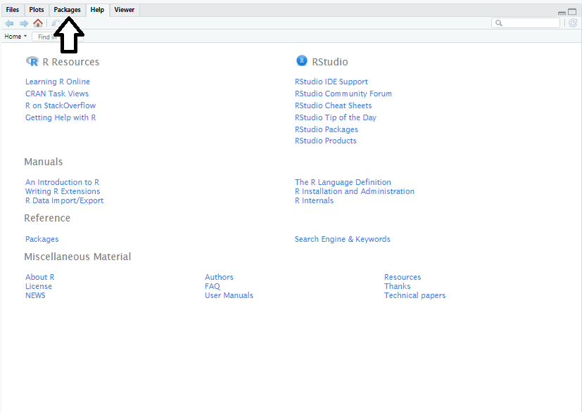
2.) Once under the ‘Packages’ Tab, click on the button labeled ‘Install’.

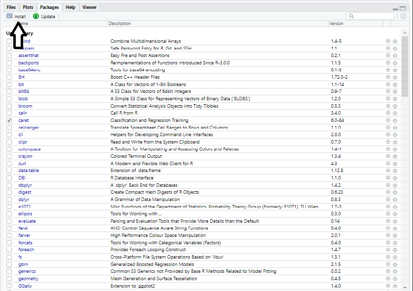
3.) A popup will open in the middle of your screen. All you have to do now it type the name of your package and click ‘Install’. In our case, we will type “caret”.

OR

1.) Type install.packages(“caret”) into the Console (bottom-left section of Rstudio)

Part Two – Introducing the ‘caret’ Package

Now that we have successfully installed the ‘caret’ package and called it using the library function, it is time to talk about what the ‘caret’ package really is. “Caret” stands for Classification And REgression Training. The package contains functions that can be used for pre-processing data, data splitting, machine learning, and many other things. However, I will be focusing on just one function in this post, the ‘train’ function. This function can be used to create and tune several different models with ease.

Part Three - Preparing our data

For this example, I want to use the Olive Oil dataset. This data is a great example for newcomers to Machine Learning due to its simplicity and how well the variables predict one another. You can gain access to this dataset by installing and calling the package “pdfCluster”. Follow the same instructions from part 1, simply changing “caret” to “pdfCluster” to do this. Now that we have installed the package and called it using the ‘library’ function we will type and execute:

data(oliveoil)

Which will put the data into our environment, readying it for use. Now let’s inspect our data. This is always a very important step! You do not want to fit any models without having an idea of what the data looks like! Type and run the following code:

str(oliveoil)

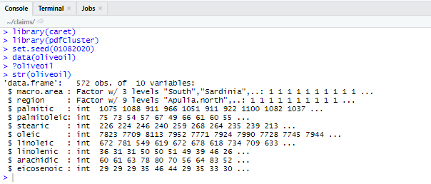
?oliveoil

Which will open up a help page on the bottom right section of RStudio. If you ever confused on how to use any dataset or function, remember that you can pull up a help page by putting a “?” in front of the function/dataset and executing the code.

Our next step will be to split the dataset into two smaller datasets to be used in Part Four. One dataset will be used to “train” our model while the other will be used to test our model’s accuracy. This is something that you will have to do for any dataset that you plan on using for Machine Learning. It is generally recommended to use roughly 75% of the data to train the model while using the other 25% for testing, however it is up to you how you want to split it up. It is also recommended to set a “seed” before you do this.

Setting a seed is a good way to get consistent random output accross multiple computers, useful if you want to follow along and get the same output as me in this demonstration. Use the following code to split up your data into separate training and testing datasets, while setting a random seed:

set.seed(01082020)
training_index <- sample(1:nrow(oliveoil), .75*nrow(oliveoil))
training <- oliveoil[training_index, ]
testing <- oliveoil[-training_index, ]

Now that we have done that, let’s breakdown what each line of code accomplished here.

Setting a seed

set.seed(01082020)

This code will set a random seed. I chose to use the date as the seed when I was writing this, but any seed would have been fine.

Generating a random sample

training_index <- sample(1:nrow(oliveoil), .75*nrow(oliveoil))

This code generates a random sample that will be used in next lines. 75% of numbers from 1 to 572 (the number of observations in our data) will be randomly selected here.

Creating our training dataset

training <- oliveoil[training_index, ]

This code will use the training index randomly generated above to assign 75% of observations to our training dataset.

Creating our testing dataset

testing <- oliveoil[-training_index, ]

This code will assign all observations not in to the training dataset to the testing dataset.

Part Four - Using the ‘caret’ package

Let’s say that you want to use the chemical measurements of an olive oil to determine which region in Italy it comes from. This is where the ‘caret’ package comes into play. We can use over 50 different methods to fit models to our data using this package. A full list of models we can fit can be found here.

For this example, I will be fitting a Random Forest model. A Random Forest model constructs a multitude of different decision trees with ‘M’ amount of variables, which are chosen randomly. When using this model for classification, whichever class has the most decision trees “voting” for it will be the class chosen by our model. ‘M’ is chosen by us, and the values it can take are integers from 1 to the total # of predictor variables. So, for this example, ‘M’ can take on any value from 1 to 8. Since this post is more about general use of the caret package, rather than Random Forest models, I will leave the description of the model there. If you would like to learn more about Random Forest models, I recommend reading an introduction here.

Now lets begin our first Machine Learning query! Type and execute the following code:

rf_model <- train(region ~. -macro.area , 
                  method = "rf", 
                  data = training, 
                  tuneGrid = data.frame(mtry = 4))
rf_model

Let’s take a close look at what we just did so I can describe what each code chunk does.

Choose our variables

region ~. -macro.area

This code determines our response and predictor variables that we would like to use in our model. On the left side of the “~”, we have region, which sets it to be our response variable. On the right side of the “~”, we are choosing our predictor variables. The “.” Indicates to the computer that we would like to use all of the remaining variables to predict our response variable. However, one of our remaining variables, “macro.area”, is just a superset of the variable “region”. We do not want to use this in our model because we established that we only want to use the scientific measurements to determine the region. I type -macro.area to indicate that I do not want that variable to be used in our model.

Select our model

method = "rf"

This code chunk determines what model we want to use. “rf” stands for Random Forest.

Choose our dataset

data = training

This is where we tell the function what dataset we want to use to train the model. We choose the “training” dataset that we created earlier.

Set model parameters

tuneGrid = data.frame(mtry = 4)

This is where we set model parameters. In a Random Forest model, there is only one parameter that we need to set, ‘mtry’. As stated before, ‘M’ is the # of variables that each decision tree will randomly select to create their model. I set mtry = 4 for this example, but you can try other numbers from 1 to 8 if you would like. One thing that is important to note is that this line of code will be different for every method you use. Different methods/models have different parameters that we need to set (some require none). Once again, I recommend using the “?” function to get help to figure out what parameters you need if you try to fit a different model.

Part Five – Testing our model

Congratulations! You have created your first model using machine learning! That model we created was stored into the rf_model variable and ready for use! Now let’s test and see how well it predicts the macro area an olive oil was created in. The go-to way to test classification models is to look at its misclassification rate when we use it to predict our test dataset we created earlier. Type and execute the following code to find your model’s misclassification rate when used on our test dataset:

misclass_rate <- (1 - mean(testing$region == predict(rf_model, testing)))*100
misclass_rate

Heres how this query works: The predict(rf_model,testing) code chunk will use our model to create classifications for our test dataset. In order to test if those classifications were accurate, I use the " == " operator to check if our predicted classes are equal to the real classifications. Taking the mean of this will give us what percentage of classifications were correct, and of course since we are looking for a misclassification percentage and not the percentage that were correctly identified, we subtract the mean from 1 and multiply by 100 to get our result.

My model returned around a 4% misclassification rate for our data. That means that I was able to correctly classify over 95% of our observations in our test dataset! If you are satisfied with your model you can stop there, or you can adjust the model parameters until you find the lowest possible misclassification rate. This process is know as tuning your model. After you are finished tuning, you are ready to use your model to predict new data!

Machine Learning has many uses here at IEL and nearly every industry in the world. The ‘caret’ package in R is equipped with a great way to implement those Machine Leaning uses to help tackle issues and predict future outcomes. I hope this demonstration was able to help get your feet into water of the deep sea of Machine Learning!